Combining 1901-1920 Temperature Anomaly and Ocean Temperature Variations in the Turn of the 20th Century: Reconstruction Based on Co-Located Land and Coastline Grid Cells
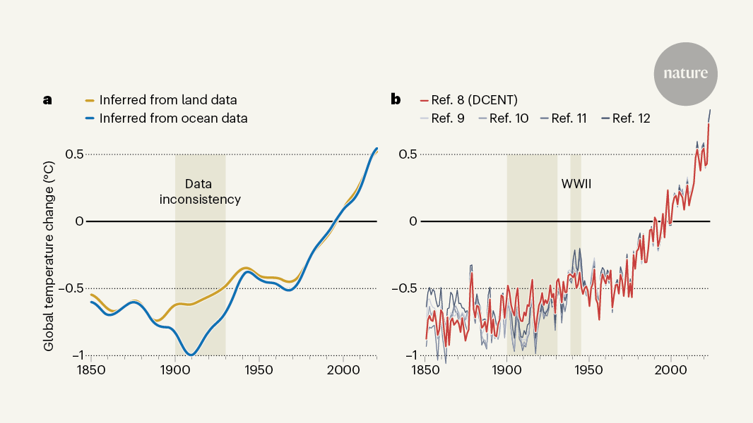
1901–1920 averages are compared with 1871–1890 averages. Because ocean-derived temperatures deviate from the land-derived temperatures from the 1890s onwards, we compared the multidecadal period before the ocean cold anomaly (1871–1890) with a period during the cold anomaly (1901–1920). We computed multidecadal temperature changes around the turn of the twentieth century as the difference between temperature averages in both periods, (\Delta {\widehat{{\bf{T}}}}^{{\rm{GMST}}}=\overline{{\widehat{{\bf{T}}}}{1901-1920}}-\overline{{\widehat{{\bf{T}}}}{1871-1890}}). The temperature differences are computed by the co-located coastal SST and LSAT data. All large-scale regions were tested for differences between co-located coastal land and coastal marine grid cells. 3c.
From these perturbed climate model patterns, we train our statistical model as indicated in equations (2) and (3), that is, to optimally predict the simulated (unperturbed) target metric (({{\bf{Y}}}{{\rm{mod}}}^{{\rm{GMST}}})). The perturbed data yields a new set of regression coefficients. Adding the error terms makes the program more accurate in its predictions of the target metric, and takes into account uncertainties and biases in the estimation of the regression coefficients. This results in lower coefficient weights for grid cells that are strongly affected by uncertainties and biases (Extended Data Fig. 2). Finally, following equations (4) and (5), we obtain observation-based reconstructions of each target metric (({\widehat{{\bf{T}}}}{{\rm{CRUTEM}}5}^{ {\rm{GMST}}}) and ({\widehat{{\bf{T}}}}_{{\rm{HadSST}}4}^{ {\rm{GMST}}})), and analogously based on CMIP6 models (({\widehat{{\bf{T}}}}{{\rm{CMIP}}6,{\rm{Land}}}^{ {\rm{GMST}}}) and ({\widehat{{\bf{T}}}}_{{\rm{CMIP}}6,{\rm{Ocean}}}^{ {\rm{GMST}}})). An ensemble of 200 observational reconstructed time series (({\widehat{{\bf{T}}}}{{\rm{CRUTEM}}5}^{ {\rm{GMST}}}) and ({\widehat{{\bf{T}}}}_{{\rm{HadSST}}4}^{ {\rm{GMST}}})) is thus obtained, where the input for each reconstruction contains a different error realization. For simplicity of notation, we dropped the parentheses in the main text, as observations-based reconstructions are trained with bias and uncertainty added to CMIP6. For the CMIP6 reconstructions. 2d,e model members have a random error and bias realizationadded to them. The reconstruction uncertainty ranges in Figs. 1 and 2 are based on the reconstructions ensembles obtained as described above (that is, conditional mean predictions based on our statistical models from 200 different bias and uncertainty realizations). An illustration of the performance of our statistical reconstruction on CMIP6 models based on sparse coverage (June 1895 for land and ocean, respectively), and more extensive coverage (June 1995 for land and ocean, respectively) is shown as Extended Data Fig. 3. An evaluation of the approach with and without uncertainties and biases is provided in Supplementary Information.
There are a number of available samples. The estimate of the regression slope is given by the minimization. The prediction error of linear regression is given.
Reconstruction of the seafloor temperature using a weighted method: The ocean versus the land based reconstruction for region-scale SST anomalies
The ocean’s temperature is different than land’s. We analysed the difference between the ocean- and land-based reconstructions at each time step for a given target metric, (\Delta {\hat{{\bf{T}}}}{{\rm{O}}\text{-}{\rm{L}}}^{{\rm{G}}{\rm{M}}{\rm{S}}{\rm{T}}}={\hat{{\bf{T}}}}{{\rm{H}}{\rm{a}}{\rm{d}}{\rm{S}}{\rm{S}}{\rm{T}}4}^{{\rm{G}}{\rm{M}}{\rm{S}}{\rm{T}}}-{\hat{{\bf{T}}}}_{{\rm{C}}{\rm{R}}{\rm{U}}{\rm{T}}{\rm{E}}{\rm{M}}5}^{{\rm{G}}{\rm{M}}{\rm{S}}{\rm{T}}}). The observationally derived Delta widehatbfT_rmOtext-rmLrmGMST was compared with the equivalently masked reconstruction range of ocean and land temperatures.
We analysed the regional SST reconstruction 33, which was based on only ocean proxy records. The ocean proxy records are derived exclusively from annually or seasonally resolved tropical coral archives. The temperature estimation is based on the Oxygen isotopic composition of the coral carbonate, but also on the skeletons of the coral and the growth rate. Reconstruction targets are regionally averaged tropical SST anomalies at the annual timescale for four large-scale ocean basins: the western Atlantic, the eastern Pacific, the western Pacific and the Indian Ocean. The study uses a weighted method to address the changing number of available observations. The paleoclimate proxies are weighted. Each record’s contribution to the composite is scaled by its relationship with instrumental target SST anomalies, considering both magnitude and significance of variance. An ensemble of reconstructions accounts for uncertainties in the CPS method, different weighting schemes and calibration periods. The ‘best’ reconstruction is selected based on the highest cumulative reduction of error score over the validation period. Finally, we analysed individual palaeoclimate proxies in Extended Data Fig. 6 and Supplementary Information.
Timescale filters and an Attribution method are used to analyse our GMST reconstructions. A low-pass and high-pass filter is used to separate our reconstruction in a low-pass and high-pass time series.
Recent studies used computers to train for optimal infill of incomplete observations. State-of-the-art climate models indeed represent key modes of ocean–atmosphere variability and forced response patterns30. The training and the testing distribution are assumed to follow the same probability distribution. This is also assumed in the method of reconstruction outlined above. Climate models don’t represent the measurement uncertainties and biases in the observed temperature record. If those uncertainties and biases were disregarded, our reconstruction algorithm would risk being ‘overfitted’—that is, too specifically tailored—to climate model simulated patterns and variability. Even though the relationship between local predictors and GMST is correct in the climate model, it would perform badly on observations. Covariate shift in statistical learning51 is a phenomenon. In the tropics, grid cells can carry high signals for estimating global-scale variability but are not always the same in the early observational record. In addition to the reconstruction method described by equations (1)–(5), we account for measurement uncertainties and biases in our reconstruction by making use of the existing, comprehensive uncertainty and bias models for CRUTEM5 and HadSST4. There are different components to the uncertainties in HadSST4 such as prevalent systematic errors with a complex temporal and spatial correlation structure. The three error terms are treated as statistically independent. The ensemble represents the different realizations of the time–space systematic errors. The errors are represented by spatial error covariance matrices and uncorrelated errors are estimated as error fields.
Observation-based predictions for all metrics were obtained after the regression coefficients had been deduced, using the spatially incomplete CRUTEM5 and HadSST4 data as inputs. The comparison of our observation-based reconstruction with CMIP6 models in Fig. 2 was based on 602 CMIP6 historical simulations that contain ‘tas’ and ‘tos’ data, that is, 98.835 model-years (overview in Supplementary Table 4), which were masked and reconstructed with observational coverage for each time step.
For the training of our regression models, we selected three historical ensemble members from each CMIP6 model, and the time period 1850–2020 (historical simulations and SSP2-4.5 simulations are concatenated up to 2020). The training dataset consisted of a total of 15,626 model-years and an overview of the CMIP6 models used for training is in Supplementary Table 4. As the optimal reconstruction coefficients may vary seasonally, training of the regression models for each month m was based on monthly data only from the same month in CMIP6 models (that is, the 15,626 model-years correspond to 15,626 monthly training samples).
The variables tas and tos are derived from climate model historical and simulations of the shared socio economic pathway. All simulations were regridded to a regular 5 × 5° longitude–latitude grid, which is identical to the CRUTEM5 and HadSST4 grid. All climate model data were centred based on a 1961–1990 reference period, in accordance with CRUTEM5 and HadSST4 data processing.
We used a standard cross-validation approach to determine the ridge regression parameter (λ) and to obtain the regression coefficients. Data science involves dividing the raw dataset into different folds. This makes sure that modelfitting and validation occur on the data subsets they are on. In the context of climate science, the cross-validation method used here adopts a ‘leave one model out’ strategy, resembling an iterative perfect model approach. In this process, for a total of k CMIP6 models, the ridge regression model is iteratively fitted on k − 1 models and validated on the kth model (referred to as ‘leave-one-model-out cross-validation’). The iterative approach guarantees that the regression coefficients generalize effectively to an unseen model, ensuring the robustness of the statistical model in the CMIP6 archive. The tuning parameter λ is then selected during cross-validation to minimize the mean squared error on out-of-fold data, and the corresponding regression coefficients are extracted. The final set of regression coefficients is obtained as the average across the k model fits. Each climate model gets its own weight for the regression in comparison to the number of ensemble members in that model.
The small yet non-zero regression coefficients are evenly distributed among the predictors. The tuning parameter λ determines the extent of shrinkage and is determined through cross-validation, as discussed in the following paragraph. The linear model’s intercept is not shrinked.
mathoprmarmrrmgrmmrmirmnlimits
Equation (1) represents a linear regression problem with a relatively high dimensionality, where the number of predictors p can be substantial (for example, p > 1,000). Ordinary least squares aim to minimize the residual sum of squares. However, in high-dimensional settings, relying on this single objective may be problematic because regression coefficients lack proper constraints53. To address such collinearity issues, we turn to ridge regression, a statistical learning technique designed for such scenarios23,53. Ridge regression prevents overfitting by incorporating a penalty for model complexity through the shrinkage of regression coefficients. The degree of the shrinkage is determined by the sum of squared regression coefficients and ridge regression coefficients. Ridge regression addresses the joint minimization problem.
Source: Early-twentieth-century cold bias in ocean surface temperature observations
HadCRUTEM5 Uncertainties Realized via the HadSST4 Ensemble and Determination of the Associated LSAT and SST Biases
$${\widehat{{\bf{T}}}}{{\rm{CRUTEM5}}:1895\text{-}06}^{{\rm{GMST}}}={X}{{\rm{CRUTEM5}}:1895\text{-}06}\,{\widehat{{\boldsymbol{\beta }}}}_{{\rm{Land}}:1895\text{-}06}^{{\rm{GMST}}},$$
The method given in Ref. is used toEncode uncertainties in CRUTEM5. There are 52. A 200-member ensemble of potential realizations of known, temporally and spatially correlated uncertainties in near-surface air temperature has been produced as part of the HadCRUT5 Noninfilled Data Set13 (that is, ϵb,Land(s, t)). The corresponding ensemble of CRUTEM5 LSAT anomalies has been extracted from this, using the HadSST4 ensemble to unblend SST and LSAT anomalies in coastal grid cells. The ensemble realization of biases encompasses uncertainties such as station-based homogenization errors and uncertainty in climatological normals, as well as regional urbanization errors and non-standard sensor enclosures (full description provided in refs. 13,40,52. Uncorrelated uncertainties can be found in the form of gridded error fields.
$${\widehat{{\bf{T}}}}{{\rm{HadSST}}4:1895\text{-}06}^{{\rm{GMST}}}={X}{{\rm{HadSST}}4:1895\text{-}06}\,{\widehat{{\boldsymbol{\beta }}}}_{{\rm{Ocean}}:1895\text{-}06}^{{\rm{GMST}}},$$
After estimating the regression coefficients, we predicted each target metric at each time step based on SST or LSAT observational datasets, and the actual coverage. LSAT and SST predictions of GMST in June 1895 would be read as such.
rLand:1895text-06