The dimensionality of the KC activity: a proofread connectome based on microtubule-free twigs

Only two values, either 0 or 1 or 1 and, are included in the matrix. In a way, this helps when calculating analytical results for the dimensionality of the KC activities. However, it is unrealistic as the connectomics data give the number of synaptic connections between the ALPNs and the KCs.

It is unclear whether the simple linear rate model presented in the original paper represents the behaviour of the biological neural circuit well. Furthermore, it remains unproven that the ALPN-KC neural circuit is attempting to maximize the dimensionality of the KC activities, albeit the theory is biologically well motivated (but see refs. 49,50).

The number of unique odour channels that each KC receives input from was solely based on their synaptic connections. We looked at how many of the 58 antennal lobes glomeruli a KC gets input from and also looked at their inputs from uniglomerular ALPNs. The K is reported based on non-thresholded connections. Filtering out weak connections does lower K but, importantly, our observations (for example, that KCg-m cells have a lower K in FlyWire than in the hemibrain) are stable across thresholds (Extended Data Fig. 7g).

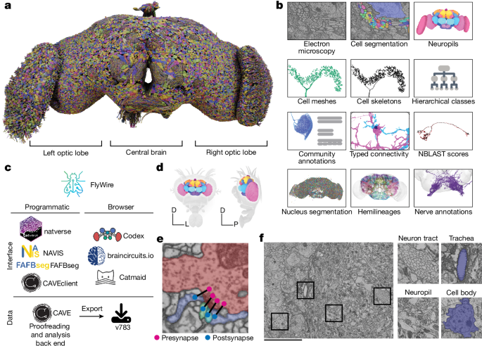
The backbones of the neurons were the focus of the proofread connectome. Microtubule-free ‘twigs’ were only added if discovered incidentally or sought out specifically by members of the community. Users marked neuron segments as complete after they had been edited, signalling that they were ready for analysis. The majority of the segments were edited by professional proofreaders in the manner used by members of the FlyWire community. First, we proofread all segments with an automatically detected nucleus in the central brain88 by extending it as much as possible and removing all false mergers (pieces of other neurons or glia attached). Second, we proofread the remaining segments in descending order of their synapse count (pre+post) up to a predefined size threshold of 100 synapses. If the remaining segments had at least one connection with at least 15 ossifications, we would check them out.

To assess quality, a group of expert centralized proofreaders conducted a review of 3,106 segments in the central brain. These specific neurons were chosen based on certain criteria such as significant change since being marked complete and small overall volume. An additional 826 random neurons were included in the review pool as well. The proofs were unaware that the neurons were added for quality measurement. We compared the 826 neurons before and after the review and found that the initial reconstruction scored an average F1-Score of 99.2% by volume (Extended Data Fig. 2a,b F1-Score is defined as the mean of recall and precision, with precision, and as the ratio of true positives and false positives among all true elements.

The top 100 players from Eyewire, a gamified electron microscopy reconstruction platform that crowdsources reconstructions in mouse retina and zebrafish hindbrain125, received an invitation to beta test proofreading in FlyWire. A new set of user onboarding and training materials were created for citizen scientists, including: a blog, forum and public Google docs. We created bite-sized introduction videos, a comprehensive FlyWire 101 resource, as well as an Optic Lobe Cell Guide to aid users in understanding the unique morphology of flies. After the introduction of players to the project by a virtual Citizen Science Symposium, theFlyers began developing their own resources, such as a new visual guide to cell types, literature reviews, and even FlyWire plugins. As of publication, FlyWire has 12 add-on apps ranging from a batch processor to cell naming helper (https://blog.flywire.ai/2022/08/11/flywire-addons/).

The robustness of hemisphere-segmentation-level morphological group annotation in the electron microstack: Application to the clustering of early-born neurons

We used the1:1 and 1:many, but did not use the many:1 matches. For the analysis of the connection stereotypy, 2,954hemibrain types were used.

Cell types that exist only on the left but not the right hemisphere of the hemibrain because our comparison was principally against the right hemisphere.

The skeletor was used to generated skeletons for all the neurons that were marked as proofread. In brief, neuron meshes from the exported segmentation (LOD 1) were downloaded and skeletonized using the wavefront method in skeletor. The skeletons were further processed, including removing false twigs and heal breaks, and produced down samples using navis128. The modified version of the skeletonization software is implemented in fafbseg.

To test the robustness of the morphological groups, we reran the above analysis across one, two or three hemispheres. The results were slightly different when this treatment was used. The persistent clusters are a group of cells that co-cluster on different hemispheres. Early-born neurons, which are often morphologically unique, frequently failed to participate in persistent clusters, and were omitted from further analysis. The Tubu neuron from the right and left hemispheres would fall when FlyWire was clustering together for hemilineage. Morphological groups are therefore defined by consistent across-hemisphere clustering. When the volume of the hemibrain was sufficient to contain the hemilineage’s cells, all of the hemispheres from FlyWire and hemibrain were used. A small number of the hemilineage- annotated neurons do not have a morphological group, as we prioritized consistency across the 3 hemisphere clustering. For example, if neuron type A clusters with type B in one-hemisphere clustering, but clusters with type C (and not B) in two-hemisphere clustering, then type A will not have a morphological group annotation.

The methods described in this section are related to the electron microscope stack. We applied a transformation to all synapses to map them into the FlyWire FAFB14.1 space. The vector field for the transformation had a resolution of 64 × 64 × 40 nm.

The navis and the natverse implement the theoretical methods used in theNBLAST. However, we modified the navis implementation for more efficient parallel computation in order to scale to pools of more than 100,000 neurons. The entire matrix of FlyWire neurons alone contains over 500 MB of memory. Most of the large NBLASTs were run on a single cluster node with 112 CPUs and 1 TB RAM provided by the MRC LMB Scientific Computing group, and took between 1 and 2 days (wall time) to complete.

Hierarchical annotation and multi-connectome cell typing of Drosophila. I. Flow, superclass and cell type in the central brain

Cell classes in the central brain represent salient groupings/terms that have been previously used in the literature (examples are provided in Supplementary Table 3). For sensory neurons, the class indicates their modality (where known). For optic-lobe-intrinsic neurons cell class indicates their neuropil innervation: for example, cell class ‘ME’ are medulla local neurons, ‘LA>ME’ are neurons projecting from the lamina to the medulla and ‘ME>LO.LOP’ are neurons projecting from the medulla to both lobula and lobula plate.

Hierarchical annotations include flow, superclass, class and cell type. The flow and superclass were assigned based on a semi-automated approach followed by manual curation. See Supplementary Table 3 for definitions and the other sections for details on certain classes.

Throughout our proofreading, matching and cell typing efforts, we recorded cases of neurons that we considered to be biological outliers or showed signs of sample preparation and/or imaging artefacts.

Each neuron was defined by a single point location and its associated PyChunkedGraph supervoxel. Every 30 min, the root IDs were updated by a Python script that was based on the fafbseg package. The location of the neuron can be found in the main arbour, located within the cell body fibre, close to the neuropil, or in a different location within the nucleus. The former was preferred as segmentation errors in the cell body fibre tracts regularly resulted in the wrong soma being attached to a given neuronal arbour. These soma swap errors persisted into proofreading and resulted in the information attached to the wrong neuron being fixed.

Source: Whole-brain annotation and multi-connectome cell typing of Drosophila

Enhanced Box Plots: Identifying Neuronal Cell Types Using Persistent Identifications from the Hemibrain

Enhanced box plots—also called letter-value plots125—in Fig. 5h and Extended Data Fig. 7f are a variation of box plots better suited to represent large samples. They replace the whiskers with a variable number of letter values where the number of letters is based on the uncertainty associated with each estimate, and therefore on the number of observations. The first fattest letters are the 25th and 75th quantiles and the second fattest is the 12th and 8th quantiles. Note that the width of the letters is not related to the underlying data.

The VirtualFlyBrain database contains information relating to fly biology, especially the topic of neuroscience. Those from the hemibrain are included in the majority of published neuron reconstructions. Each individual neuron (that is, one neuron from one brain) has a persistent ID (of the form VFB_xxxxxxxx). When cell types have been defined, they have an ID, like the one for DNa02 DN. Importantly, VFB cross-references neuronal cell types across publications even if different terms were used. It also identifies driver lines to label many neurons. In this paper, we provide the closest and fine-grained term that is already in their database with an initial mapping. For example, a FlyWire neuron with a confirmed hemibrain cell type will receive a FBbt ID that maps to that exact cell type, while a DN that has been given a new cell type might only map to the coarser term ‘adult descending neuron’. Work is already underway to assign the VFB IDs to FlyWire cell types, and to all individual FlyWire neurons.

A Statistical Analysis of the FlyWire Dataset for the Study of Brain Functions and Identifying Neurons that Are Entering and Exiting the Brain

Statistical analyses such as Pearson R were performed using the implementation in the scipy123 Python package. We used either a t-tests for normally distributed samples, or a Kolmogorov–Smirnov test.

The number of input connections to each mixing layer neuron is kept at a constant K for all neurons. It is possible to make it simpler by using a distribution P(K) but more detailed modelling is required.

All of the mixing layers are assumed to have a single value for global inhibition provided by APL. The level of inhibition would not be the same depending on the amount of APL and mixing layer neurons.

From Fig. When compared with the hemibrain, the shift towards the lower values of K found in the FlyWire left and FlyWire right datasets can be seen.

For consistency with visualizations and datasets obeying the standard convention (fly’s right on viewer’s left), FlyWire data can be mirrored. The tools we give to mirror data are in the form of the flybrains or natverse. 1c), through the

Seung and Murthy say that they’ve been developing the FlyWire map for more than four years, using electron microscopy images of slices of the fly’s brain. The researchers and their colleagues stitched the data together to form a full map of the brain with the help of artificial-intelligence (AI) tools.

To identify the cells that are entering and leaving the brain, weseeded all profiles in a cross section of the GNG. We found all of the DNs based on criteria: they were located in the brain, and main axon branch leaving the brain.

The following criteria were used to identify these ANs: (1) no soma in the brain, and (2) main branch entering through the neck connective as well as axon.

To identify DNs described in ref. The volume depictions of the lines were transformed into FlyWire space. Matching closely related neurons could be achieved by using the same space for displaying EM and LM neurons. We identified candidate matches by eye and transformed them into JRC 2018.U space and put them onto the GAL4 or Split GAL4 line stacks. 107 for that type) in FIJI for verification. Using these methods, we identified all but two (DNd01 and DNg25) in FAFB/FlyWire and annotated their cell type with the published nomenclature. All other unshackled DNs received a systematic cell type that included their soma location, an ‘e’ for EM type and three digit number. There is a detailed account and analysis ofDNs in the book.

We next classified the DNs based on their soma location according to a previous report107. In brief, the soma of DNa, DNb, DNc and DNd is located in the anterior half (a, anterior dorsal; b, anterior ventral; c, in the pars intercerebralis; d, outside cell cluster on the surface) and DNp in the posterior half of the central brain. The GNG contains DNg somas.

Side refers to the place in the brain where the sensory neurons enter. Some of the cases we couldn’t tell the nerve entry side from the side assigned to it.

We also note that our annotations include a number of non-neuronal cells/objects such as glia cells, trachea and extracellular matrix that others might find useful (superclass not_a_neuron; listed in Supplementary Data 2).

Using methods described in detail in the sections below, we defined cell types for 96.4% of all neurons in the brain—98% and 92% for the central brain and optic lobes, respectively. The 3.6% of neurons were mostly local cells in the brain and included a number of midline neurons.

Johnston’s organ neurons in the right hemisphere were characterized based on innervation of the major AMMC zones (A, B, C, D, E and F), but not further classified into subzone innervation as shown previously104. The left hemisphere’s sensory neurons were compared to the right hemisphere’s by using a combination of matching and expert review. The antennal brain cells were identified through the connection to uniglomerular projection neurons, and the matching to previously identified hemibrain neural cells.

Sensory neuron were cross- examined to find out how the cell type was used and whether the class field applied to it. The left hemisphere has been identified as the location of almost all of the head and taste scepters. The sensory cells were identified in ref. 103 and Johnston’s organ neurons in refs. 104,105 in a version of the FAFB that used manual reconstruction (https://fafb.catmaid.virtualflybrain.org). Those neurons were identified by transformation in the FlyWire instance.

A Search for New Hemilineage Tracts in Clusters of Connected Neurons (C/T). I. Vl5/BLva3/BL Va2c

The majority of VPNs (99.6%) and VCNs (98.3%) were assigned to specific types. Only 29 VPNs and 9 VCNs could not be confidently assigned a cell type and were therefore left untyped.

Hemibrain types split across multiple clusters were double checked (for example, by running a triple-hemisphere connectivity clustering), which often led to a split of the hemibrain type; for example, SMP408 was split into SMP408a–d.

The format for the name is called “neuropil”, where it refers to regions innervated by VPN dendrites and C/T stands for columnar versus tangential organization.

Clusters containing a mix of hemibrain-typed and untyped neurons typically meant that, after further investigation, the untyped neurons were given the same hemibrain type.

We can now reconcile previous reports if we thoroughly inspected the hemilineage tracts originally in CAmAID and then in FlyWire. New to the refs. These are the genes that we gave to the neuron line: VLPl5/BLva3_ or_4. 33,34. New to ref. SLPpl3/BL Va2c is one of the Hartenstein nomenclatures. We did not take the following clones from ref. The total count of hemilineages has not been clearly demonstrated because they are not clearly shown in the Laetus: VPNd2,vpnd3,vpnp2 andvpnp4.

There are 3 type I lineages that have more than two tracts in the clone and they are VLPp&l1/DPLpv. Without taking these type I and type II tracts into account, we identified 141 hemilineages.

coconatfly: A streamlined interface to clustering, II: hemibrain types, connections and the number of input connections

The coconatfly package provides a streamlined interface to carry out clustering. For example the following command can be used to see if the types given to a selection of neurons in the Lateral Accessory Lobe (LAL) are robust:

The optional interactive mode in the web browser can be used for efficient exploration. For further information about the examples, see https://natverse.org/.

In rare cases, clusters contained a mix of two or more hemibrain types; these were double checked and the hemibrain types corrected (for example, by merging two or more hemibrain types, or by removing hemibrain type labels).

and how it changes with respect to K, the number of input connections. I wonder what the numbers of inputs K into individual KCs mean, given that M KCs, N ALPNs and a global inhibition are involved.

More detailed calculations can be found in a previous report122. The rows in can have 1 and N K elements, as per the randomized weights used in. The parameter α represents a homogeneous inhibition corresponding to the biological, global inhibition by APL. The value was set to be, where A is a constant and M is the amount of KCs in the three datasets. The primary quantity of interest is the dimension of the KC activities defined by122:

Early Access Users of FlyWire for Early Data Access to the Production Dataset: A Field-Inspired Multi-Layer Proofreader Based on Ultrastructures

The professional team received additional training. Correct proofreading relies on a diverse array of 2D and 3D visual cues. Proofreaders learned about 3D morphology, resulting from false merger or false split without knowing what types of cells they are. The ultrastructures are reliable guides for accurate tracing and provide valuable 2D cues. Before they were admitted into Production, professional proofreaders practiced on an average 200 cells in a testing dataset where additional feedback was given. In this dataset, we determined the accuracy of test cells by comparing them to ground-truth reconstructions. Peer learning was encouraged in order to improve the quality of proofreading.

Proofreaders came from several distinct labour pools: community members, citizen scientists from Eyewire (Flyers), and professional proofreading teams at Princeton and Cambridge. Proofreaders at Princeton consisted of staff at Princeton University and at SixEleven. Similarly, proofreading at Cambridge was performed by staff at Cambridge University and Ariadne. THe built-in interactive tutorials and directions for self-guided training were given to all of the proofreaders. For practice and learning purposes, the Sandbox, a complete replica of the FlyWire data, allowed new users to freely make edits and explore without affecting the actual ‘Production’ dataset. When ready, an onboarding coordinator tested the new proofreader before giving access to the Production dataset8. Later onboarding called for users to send demonstration Sandbox edits that were reviewed by the onboarding coordinator. A new class of view-only users was introduced in early 2023, allowing researchers early data access for analysis purposes. All early access users attended a live onboarding session in Zoom prior to being granted edit or view access.

A cell that was marked complete by any user of FlyWire was a good one for analysis. As smaller branches were added later on, there was nothing that could have prevented future proofreading of a cell. We created an annotation table for these completion markings. Each completion marking was defined by a point in space and the cell segment that overlapped with this point at any given time during proofreading was associated with the annotation. We created a service where users could submit completion markings for any cell. For convenience, we added an interface to this surface directly into Neuroglancer such that users can submit completion information for cells right after proofreading (Supplementary Fig. 10). When users submitted completion annotations we also recorded the current state of the cell. We encouraged users to submit new completion markings for a cell that they edited to indicate that edits were intentional. Recording the status of a cell at submission enabled us to calculate volumetric changes to a cell through further proofreading and flag cells for review if they received substantial changes without new completion markings.

Source: Neuronal wiring diagram of an adult brain

Brain volume analysis of C. elegans: Intrinsic hemibrases and nerve ring in the ventral lobe and excretory pore

Based on their presynaptic location, we assigned the synapses to the neuropils. We used ncollpyde to calculate the location of the site and assign it to the right spot. After this step, some of the sceptics remained unassigned due to the rough outlines of the underlying data. We then assigned all remaining synapses to the closest neuropil if the synapse was within 10 µm from it. The remaining synapses were left unassigned.

We calculated a volume for each neuropil using its mesh. The paper had aggregated volumes where the medula, accessory medula, lobula and lamula plates were assigned. The remaining neuropils but the ocellar ganglion were assigned to the central brain.

$$\begin{array}{l}P\,=\,\frac{{\rm{TP}}}{{\rm{TP}}+{\rm{FP}}}\ R\,=\,\frac{{\rm{TP}}}{{\rm{TP}}+{\rm{FN}}}\ {\rm{F1}}\,=\,\frac{2\times P\times R}{P+R}\end{array}$$

The latest completion rates and synaptic numbers for hemibrain were retrieved from neuprint. The hemibrain dataset made it difficult for neuropil comparisons to be made. We excluded these regions from the comparison.

The brain of C. elegans extended from the ring-shaped structure around the pharyngealx to the excretory pore. (We follow the authors who call this region the nerve ring plus the anterior portion of the ventral nerve cord, though some authors refer to the combined structure as the nerve ring.) Nine neurons (RIR, RIV, RMDD, RMD and RMDV) are intrinsic to the nerve ring itself. An additional 26 neurons (AIA, AIB, AIM, AIN, AIY, AIZ, RIA, RIB, RIC, RIH, RIM, RIS, RMF and RMH) are intrinsic to the combined structure, for a total of 35 intrinsic neurons in the brain.

It should be understood that this estimate has ‘error bars’ because of definitional ambiguities. Ten motor neurons (RMH, RMF and RMD) could arguably be removed from the list, as it is unclear whether motor neurons qualify as intrinsic neurons. Or the brain could be enlarged by moving the posterior border further behind the excretory pore, which would add 10 neurons (RIF, RIG, RMG, ADE and ADA). 35 10 intrinsic neuronal numbers are what we estimate, so they are explicit. Of the 302 CNS neurons, 180 make synapses in the brain126. Therefore, neurons intrinsic to the brain make up about 15 to 25% of brain neurons, and 8 to 15% of CNS neurons.

We calculated cell volumes and surface areas using CAVE. Volumes were computed by counting all voxels within a cell segment and multiplying the count by the voxel resolution. Area calculations were more complicated and were performed by overlap through shifts in voxel space. The overlap of false and true voxels was obtained by shifting the binarized segment in each dimensions. The count by the voxel resolution of the given dimensions was taken to add the extracted voxels. Finally, we added up per dimension area estimates. smoothed measurements were too compute intensive and the measurement will overestimate area by a small amount.

The synapse classifier by Buhmann et al. was trained on ground truth from the CREMI challenge (https://cremi.org). The three CREMI datasets contain three 5 5 5 m cubes from the calyx. While the classifier from Buhmann et al. was trained and validated on only this dataset, they evaluated its performance on multiple regions (calyx, lateral horn, ellipsoid body and protocerebral bridge). It should be noted that performance varies by region.

Eckstein et al.10 created a machine learning model to predict neurotransmitter identities for all synapses from Buhmann et al. based on the electron microscopy imagery alone. Each neuron was assigned a chance to carry one of the six neurotransmitters. They used neurotransmitter identities published for individual neuronal cell types and built a dataset with 3,025 neurons with known transmitter type assuming Dale’s law applies. Eckstein et al. reported a per-synapse accuracy of 87% and a per neuron (majority vote) accuracy of 94%.

The left and right hemisphere presynapses are calculated for each neuron. The hemisphere opposite its dominant input side was named the contralateral hemisphere. We excluded neurons that had either most of their presynapses or most of their postsynapses in the centre region.

We used the information flow algorithm implemented by Schlegel et al.26,128 (https://github.com/navis-org/navis) to calculate a rank for each neuron starting with a set of seed neurons. The algorithm traverses the synapse graph of neurons probabilistically. The likelihood of a neuron being added to the traversed set increased linearly with the fraction of synapses it receives from already traversed neurons up to 30% and was guaranteed above this threshold. We repeated the rank calculation for all sets of afferent neurons as seed as well as the whole set of sensory neurons. The groups we used are: olfactory receptor neurons, gustatory receptor neurons, mechanosensory Johnston’s organ neurons, head and neck bristle mechanosensory neurons, mechanosensory taste peg neurons, thermosensory neurons, hygrosensory neurons, VPNs, visual photoreceptors, ocellar photoreceptors and ascending neurons.

Additionally, we created input seeds by combining all listed modalities, all sensory modalities, and all listed modalities with visual sensory groups excluded.

We averaged 10,000 runs for every modality. We placed the neurons according to their rank and assigned them a percentile based on their location. To compute a reduced dimensionality, we treated the vector of all ranks (one for each modality) as neuron embedding and calculated two dimensional embeddings using UMAP129 with the following parameters: n_components=2, min_dist=0.35, metric = “cosine”, n_neighbors=50, learning_rate = .1, n_epochs=1000.

A Flywire project to identify 8,453 types of neuron that make up an fly to stop and groom itself: A multisensory map of brain connections that tell humans how to stop

In another study3, researchers describe two wiring circuits that signal a fly to stop walking. The fly brain is responsible for sending signals to the other side of the brain when the fly wants to stop and eat. The other circuit includes neurons in the nerve cord, which receives and processes signals from the brain. The fly can stop while it grooms itself with the help of these cells.

Some of the ways in which the cells communicate was surprising to the team. For instance, neurons that were thought to be involved in just one sensory wiring circuit, such as a visual pathway, tended to receive cues from multiple senses, including hearing and touch1. “It’s astounding how interconnected the brain is,” Murthy says.

But the work wasn’t finished: the map still had to be annotated, a process in which the researchers and volunteers labelled each neuron as a particular cell type. Jefferis compares the task to assessing satellite images: AI software might be trained to recognize lakes or roads in such images, but humans would have to check the results and name the specific lakes or roads themselves. All told, the researchers identified 8,453 types of neuron — much more than anyone had expected. Of these, 4,581 were newly discovered, which will create new research directions, Seung says. “Every one of those cell types is a question,” he adds.

The map1 is described in a package of nine papers about the data published in Nature today. Its creators are part of a consortium known as FlyWire, co-led by neuroscientists Mala Murthy and Sebastian Seung at Princeton University in New Jersey.

“This is a huge deal,” says Clay Reid, a neurobiologist at the Allen Institute for Brain Science in Seattle, Washington, who was not involved in the project but has worked with one of the team members who was. The world has been waiting for something for a long time.